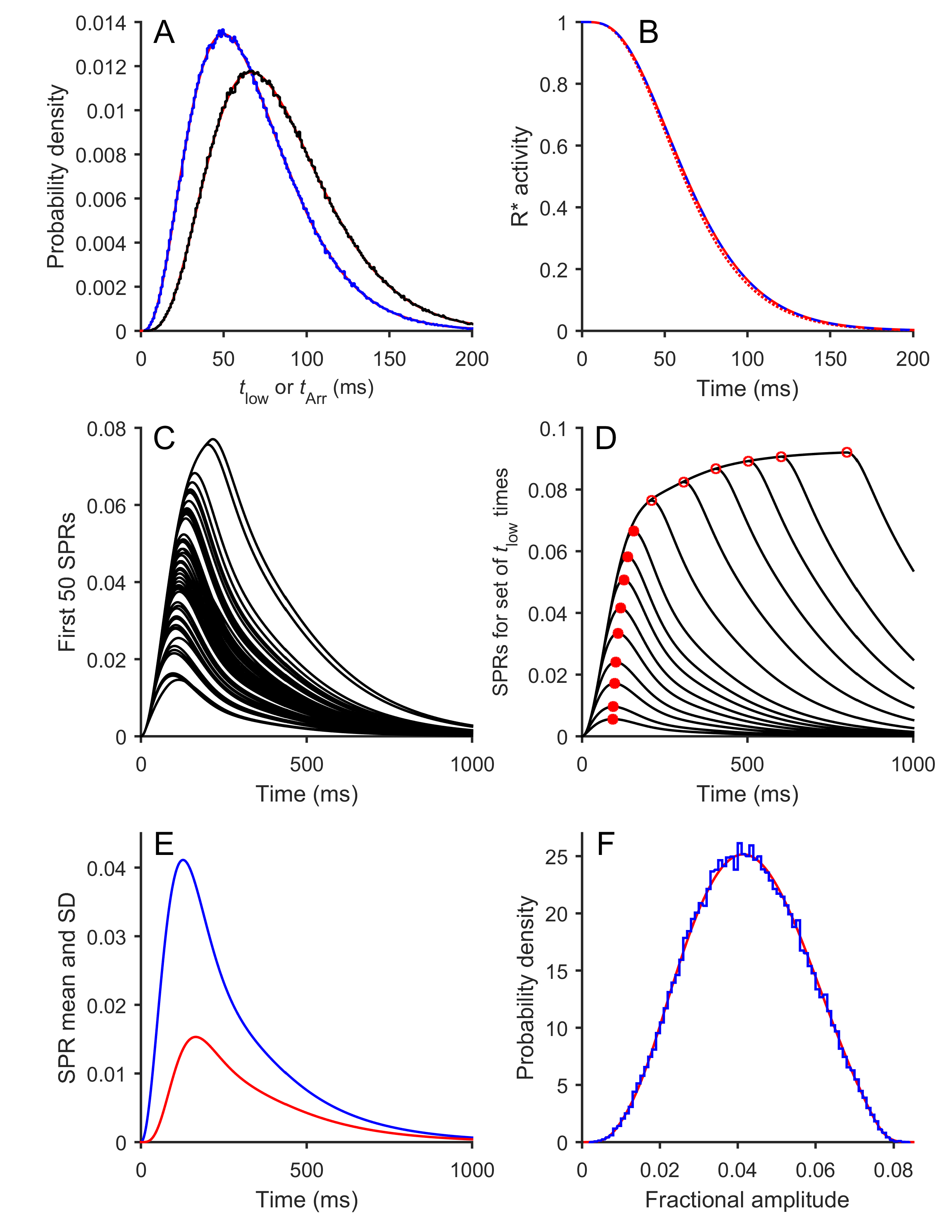
Figure 4. Results of simulation of Model 3 (Three-state model). The equations for Model 3 were simulated numerically using M = 3 and ν = κ = μ = 60 s⁻¹ for the stochastic parameters (Table 1) and with the downstream parameters from Table 2; the flash duration was set to zero. The number of simulations of R* activity in panels A and B was 10⁶, while for the subsequent panels the downstream reactions were integrated using the first 50 R* simulations (panel C) or the first 10⁵ R* simulations (panels E and F). A: Distribution of times to the low-activity state (left) and to Arr binding (right) for the 10⁶ simulations. Blue traces are simulations, and red curves are theoretical predictions. B: Mean R*(t) time-course, for the 10⁶ simulations (dashed blue trace). The overlying dashed red trace is the prediction of Equation (3.5). For comparison, the dotted red trace shows the predicted response for the binary model using the same values of ν and μ; thus it plots the dashed red trace from Figure 3B. The similarity of these traces shows that inclusion of the low-activity state made little difference to the mean time-course of the simulated and predicted R*(t) responses. C: The first 50 simulated SPRs. D: SPRs for a set of defined times to the low-activity state. Rather than being simulated stochastically, the interval until low activity was instead set to 5, 10, 20, 30, 45, 60, 80, 100, 130, 200, 300, 400, 500, 600, or 800 ms. The subsequent delay to arrestin binding was fixed at its mean value of 1/μ. Red circles indicate the peaks. These measurements were fit by a spline function and used to predict the expected distribution in panel F. E: Time course of the mean (blue) and SD (red) for the ensemble of 10⁵ simulated SPRs. F: Probability distribution of the peak amplitudes for the 10⁵ simulated SPRs (blue). The smooth red trace plots the predicted distribution obtained using the approach described in the Theory section using Equation (3.6) and the measurements of peak amplitude from panel D.