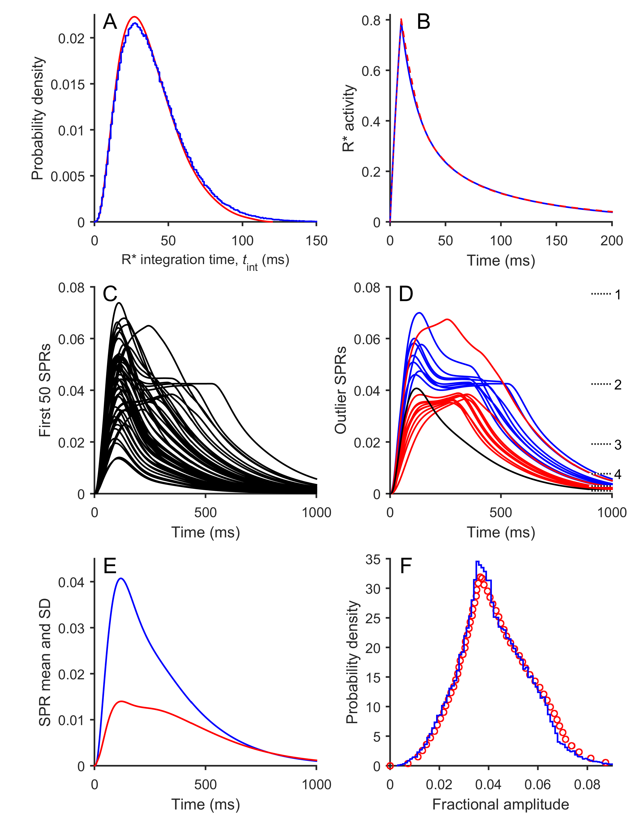
Figure 2. Results of simulation of Model 1 (Graded R* shut-off model). The equations for Model 1 were simulated numerically using stochastic parameters n = 6, M = 3, ν_max = 80 s⁻¹, μ = 20 s⁻¹, and ω_P = ω_G = 1 (Table 1); the flash duration was set to 10 ms. The downstream parameters are given in Table 2, with α_max = 150 µM/s, β_Dark = 4 s⁻¹, and β_sub = 0.063 s⁻¹. The number of simulations of R* activity in panels A and B was 10⁶, while for the subsequent panels the downstream reactions were integrated using the first 50 R* simulations (C), the first 200 R* simulations (D), or the first 10⁵ R* simulations (E and F). A: Distribution of times to Arr binding for the 10⁶ simulations (blue trace). The red trace is the corresponding curve from the simulations of Gross et al. [11] plotted in their illustration 6E. B: Mean R*(t) time course for the 10⁶ simulations (blue trace). The red trace is the corresponding curve from the simulations of Gross et al. [11] plotted in their Supplementary illustration S2C. C: The first 50 simulated SPRs. D: Sample “outlier” SPR responses, selected as described in the text from the first 200 R* simulations. Blue: The 10 SPRs with the longest times in state R*·P(2). Red: The 10 SPRs with the longest time-to-peak. The horizontal dotted lines at the right indicate the steady-state levels reached with very long dwell times in each of the states R*·P(n) . These levels have been numbered for n = 1 – 4, but are not numbered for 5 or 6. The level for state R*·P(0) is above the top of the vertical scale, at 0.114. E: Time course of the mean (blue) and SD (red) for the ensemble of 10⁵ simulated SPRs. F: Probability distribution of the peak amplitudes for the 10⁵ simulated SPRs (blue). The red circles show the corresponding histogram plotted by Gross et al. [11] for their simulations in their illustration 6E.