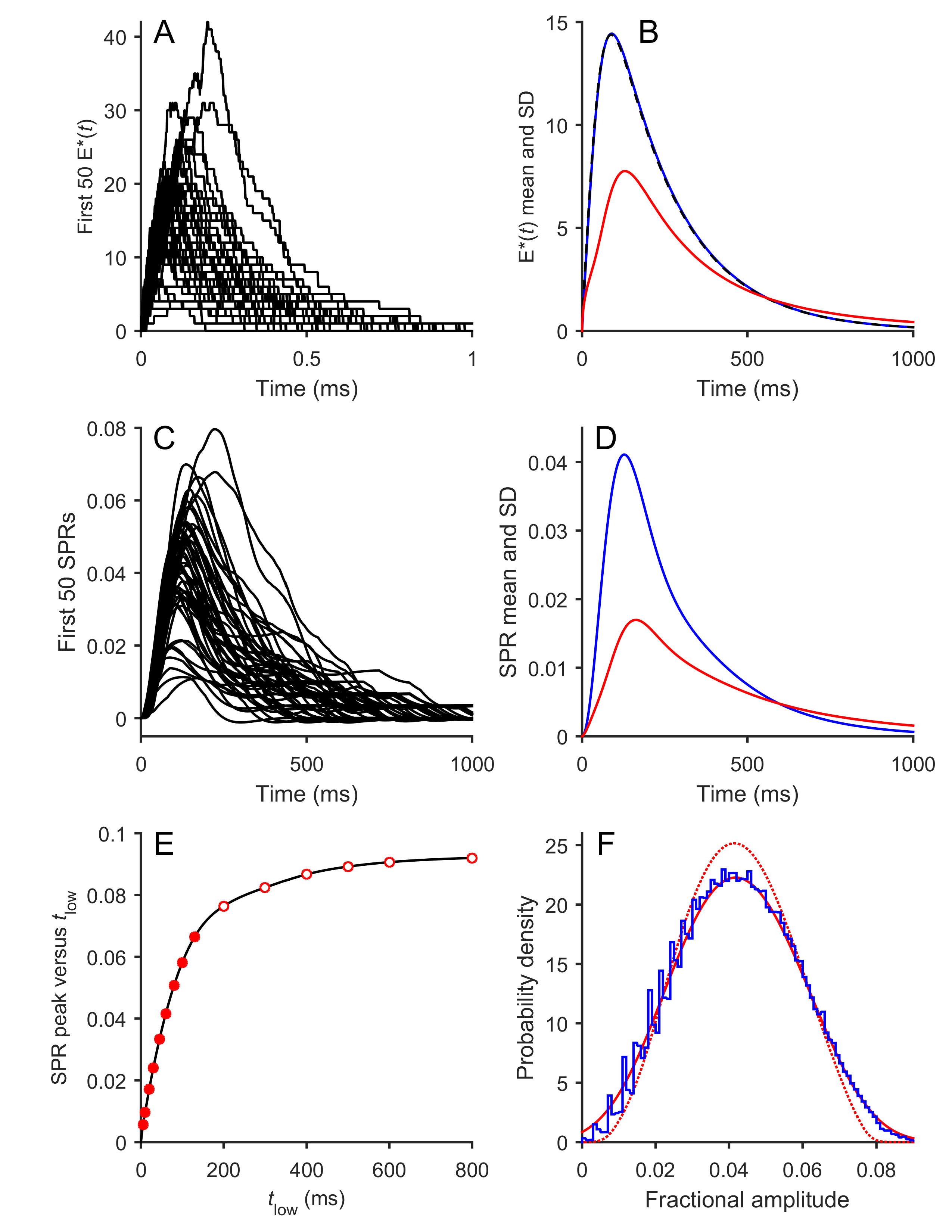
Figure 5. Stochastic generation and shut-off of E* combined with the three-state R* model. The three-state model has been extended by simulating E* generation and shut-off as being stochastic, with the same rate constants (ν_RE and k_E) as in the deterministic E* case in Figure 4. All other features of the simulation were identical to those in Figure 4, including the seed for the random number generator, so that the sequence of R*(t) simulations was the same. A: The first 50 simulations of E*(t). B: Mean (blue) and SD (red) of the E*(t) time-course for the 10⁵ simulations. The dashed black trace is the predicted mean E*(t) time-course, obtained by convolving the mean R*(t) time-course with the deterministic E* impulse response, ν_RE exp(−k_E t). C: The first 50 simulations of SPRs. D: Mean (blue) and SD (red) SPR time course for the 10⁵ simulations. E: Relationship between SPR amplitude and t_low from Figure 4D. Symbols plot the measured SPR peak amplitudes, and the curve is a spline fit. F: Probability distribution of the peak amplitudes for the 10⁵ simulated SPRs (blue). Minor peaks are visually resolvable for what we presume to be the first eight E*s. The dotted red trace is redrawn from the red trace in Figure 4F, while the continuous red trace is the convolution of the dotted trace with a Gaussian function representing variability of the number of E*s; see Text.