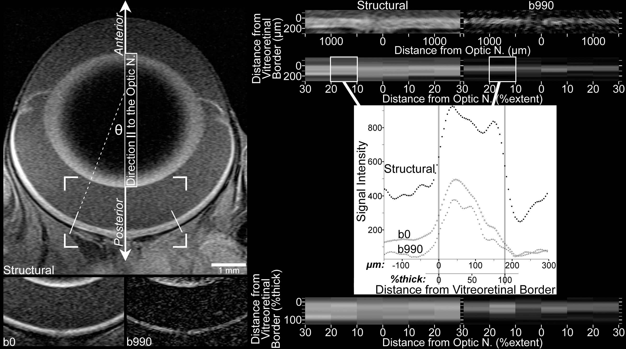
Figure 1. Image processing included linearization of the central retina, followed by spatial normalization according to location along
the extent of the retina (‘%extent’) between the optic nerve (at 0%extent) and ciliary body (at 100%extent), and location
within the thickness of the retina (%thick) between the vitreoretinal border (at 0%thick) and the retina-choroid border (at
100%thick).
Top left: Structural image shows the orientation of the eye relative to the direction parallel to the optic nerve (║) and anterior/posterior
orientation. Only the central retina is analyzed, from 10% to 30% of the hemiretinal extent (the distance, measured along
the vitreoretinal border, from the optic nerve to the ciliary body). The 30%extent boundaries are indicated by solid white
lines angled perpendicular to the vitreoretinal border. Cell structures of interest within the retina include the rod outer
segments, which are found in the posterior outer retina and have their long axis oriented radially, relative to the center
of the eye (parallel to incident light). Although the curvature of the eye produces measurements of apparent diffusion coefficient
parallel to the optic nerve (ADC║) that include structures (e.g., photoreceptors) oriented off-║ by ≤θ, this should have negligible
impact on ADC comparisons (see Discussion).
Bottom left: Cropped images (the corners of the cropped region are overlaid on the structural image above) collected with b=0 and b=990
s/mm
2 in the ║ direction. For display purposes, brightness and contrast settings are the same for all b0 and b990
║ images in this figure, but a different pair of brightness and contrast settings is applied to structural images. Due to resampling
and averaging steps used to produce the b0 and structural images (see Methods), the b990
║ image best displays the native spatial resolution of diffusion images.
Top right: The linearized central retina from the structural and b990
║ images is shown here. Since the vitreoretinal border smoothly follows the curvature of the eye, its location can be determined
with accuracy in excess of the native spatial resolution: Using the images on the
left, the approximate location of the border is found in several neighboring columns of voxels. A polynomial best fit to these
locations specifies the vitreoretinal border. Linearized images are produced by sampling every 4.63 μm along perpendiculars
to those high-order polynomials. Data in the linearized images is binned by retinal extent, and averaged within each bin.
This spatial averaging improves signal-to-noise before diffusion calculations, and since it is done on linearized images,
the critical spatial information—distance from the vitreoretinal border—is well preserved.
Mid right (plot): Signal intensity data from the left 10%–20%extent bin is plotted to show the location of vitreoretinal and retina-choroid
borders, which are determined in structural data using the half-height approach (i.e., the border is at the halfway point
between local minimum and maximum) [
20]. The same borders are found in the b0 profile, and are used to align b0 and structural images. As detailed extensively in
previous work [
4], data collected with b≥0 are then aligned to b0 data using the broad signal peak in the anterior approximately one-half
to two-thirds of the retina (visible here from approximately 0 to 100 μm).
Bottom right: As previously described [
19], after the retinal thickness is calculated by subtracting the vitreoretinal and retina-choroid borders, the data are resampled
according to distance from the vitreoretinal border relative to the retinal thickness. Finally, the resampled data (within
each %extent bin, one value every 4%thick) from 10%–30%extent on each side of the optic nerve are averaged to produce a single
profile, which is used for within- and across-subjects comparisons.
 Figure 1 of
Bissig, Mol Vis 2012; 18:2561-2577.
Figure 1 of
Bissig, Mol Vis 2012; 18:2561-2577.